


APA
ISO 690-2
Harvard
Haga clic en un formato de citación
Bayesian Evaluation for Uncertainty of Indirect Measurements in Comparison with GUM and Monte Carlo*
Evaluación bayesiana de la incertidumbre en mediciones indirectas comparada con GUM y Monte Carlo
Juan Daniel Molina-Muñoz, Luis Fernando Giraldo-Jaramillo, Edilson Delgado-Trejos
Bayesian Evaluation for Uncertainty of Indirect Measurements in Comparison with GUM and Monte Carlo*
Ingeniería y Universidad, vol. 26, 2022
Pontificia Universidad Javeriana
Juan Daniel Molina-Muñoz a juan.molina@cimat.mx
Centro de Investigación en Matemáticas CIMAT, México
Luis Fernando Giraldo-Jaramillo
Instituto Tecnológico Metropolitano ITM, Colombia
Edilson Delgado-Trejos
Instituto Tecnológico Metropolitano ITM, Colombia
Received: 08 december 2019
Accepted: 17 march 2021
Published: 13 july 2022
Abstract: Objective: To propose a methodological procedure that serves as a guide for applying techniques in the measurement uncertainty evaluation, such as GUM, MMC, and Bayes; in addition, to develop an application in a non-trivial case study. Materials and methods: In this paper, a set of steps are proposed that allow validating the measurement uncertainty evaluation from techniques such as GUM, MMC, and Bayes; these were applied as a strategy to evaluate the uncertainty of an indirect measurement process that sought to determine the level of a fluid by measuring the hydrostatic pressure generated by it at rest on the bottom of a container. The results obtained with each technique were compared. Results and discussion: the use of the GUM was found to be valid for the case under study, and the results obtained by applying the Bayesian approach and the MC technique provided highly useful complementary information, such as the Probability Density Function (PDF) of the measurand, which enables a better description of the phenomenon. Likewise, the posterior PDF obtained with Bayes allowed us to approximate closer values around the true values of the measurand, and the ranges of the possible values were broader than those offered by the MMC and the GUM. Conclusions: In the context of the case under study, the Bayesian approach presents more realistic results than GUM and MMC; in addition to the conceptual advantage presented by Bayes, the possibility of updating the results of the uncertainty evaluation in the presence of new evidence.
Keywords:Uncertainty estimation, GUM, Monte Carlo method, Bayesian inference, indirect measurement.
Resumen: Objetivo: Proponer un procedimiento metodológico que sirva de guía para aplicar técnicas en la evaluación de la incertidumbre de medida, como son: GUM, MMC y Bayes; además, de desarrollar una aplicación en un caso de estudio no trivial. Materiales y métodos: En el presente artículo, se proponen un conjunto de pasos que permiten validar la evaluación de incertidumbre de medida a partir de técnicas como GUM, MMC y Bayes; estas se aplicaron como estrategia para evaluar la incertidumbre de un proceso de medición indirecta, donde el experimento de pruebas consistió en determinar el nivel de un fluido a través de la medición de presión hidrostática que genera el fluido en estado estacionario sobre la base de un contenedor. Se compararon los resultados obtenidos con cada técnica. Resultados y discusión: se encontró que el uso de la GUM es válido en el fenómeno caso de estudio, sin embargo, los resultados obtenidos aplicando el enfoque Bayesiano y el MMC ofrecieron información complementaria de mucha utilidad, como es la función de densidad de probabilidad (FDP) del mensurando, que permitió una mejor descripción del fenómeno. Asimismo, las FDP a posteriori obtenidas con Bayes permitieron aproximar a valores más cercanos en torno de los verdaderos valores del mensurando, y los intervalos de los posibles valores fueron más amplios que los que ofrecieron el MMC y la GUM. Conclusiones: En el contexto del caso de estudio se tiene que el enfoque bayesiano presenta resultados más realistas que GUM y MMC; además de la ventaja conceptual que presenta Bayes, de la posibilidad de actualizar los resultados de la evaluación de incertidumbre ante la presencia de nueva evidencia.
Palabras clave: Evaluación de incertidumbre, GUM, Método de Monte Carlo, Inferencia Bayesiana, Medición indirecta.
Introduction
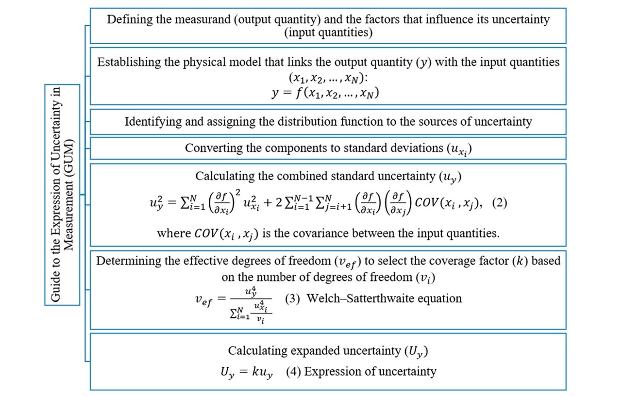
The numerical value of a measurand can be determined directly or indirectly. In both cases, the result of said measurement must include the estimated uncertainty, which, according to the Guide to the Expression of Uncertainty in Measurement (GUM), is defined as the “parameter, associated with the result of a measurement, that characterizes the dispersion of the values that could reasonably be attributed to the measurand”[1]. Measurement uncertainty is affected by certain factors that depend on the measurand, the physical phenomenon involved, the measurement protocol, and the measurement characteristics of the equipment used, among others. The aim is to quantify the contribution of each selected factor to the global uncertainty associated with the measurand, including the possible relationships between the factors. A technical expert, usually a person engaged in instrumentation or metrology, is responsible for selecting the number of factors to consider and establishing their influence on the measurand.
Traditionally, measurement uncertainty has been estimated using the GUM. However, it is not advisable to use this guide in some situations, such as: (i) when systems have very marked non-linearities or a complex behavior, i.e., when it is difficult to predict future dynamic evolution [2], and (ii) when the output quantity’s probability distribution is not normal or not easy to approximate to a normal one [3]. In these circumstances, the Monte Carlo (MC) method, based on the concept of propagation of distributions, is the preferred alternative [4]. This method assigns a Probability Density Function (PDF) to each input quantity. By means of random sampling, multiple values of these quantities are obtained, then inserted into the model, thus generating observations of the output quantity [5]. Based on these observations, a PDF for the output quantity (from which uncertainty is estimated) is constructed [6]. In [7], the authors quantified the uncertainty in measuring the volume of water delivered by a volumetric container using the GUM and the MC method. According to their results, the coverage interval of the GUM turned out to be slightly wider than that of the MC method at the same confidence level. Very similar results have been obtained with both techniques [8], although a strong dependence on the statistical nature of the measurements on the time series has been observed [9].
Alternatively, measurement uncertainty can also be estimated via the Bayesian approach [10], which is considered more natural and suitable[11]. In this approach, the parameters associated with the input quantities are assigned a prior PDF that can be based on background knowledge of the phenomenon, trends reported in the literature regarding the phenomenon [12], or previously available data [13]. Non-informative prior PDFs can also be chosen if there is not much prior information on the input quantity, thus ensuring greater objectivity [14]. Using Bayes’ theorem, the prior PDFs are combined with data obtained from experiments; as a result, posterior distributions are yielded for each of the parameters associated with the input quantities. Based on the model that links the input quantities with the output quantity and the posterior PDFs of the input quantities, the posterior PDF of the measurand is obtained, which is used to assess measurement uncertainty [15].
In [16], the authors outlined some advantages of the Bayesian approach over the GUM regarding coverage interval and probability. When there is poor or no prior information, the Bayesian approach works well, while the GUM can lead to insidious difficulties [17], [18]. When there are no dominant input quantities with Type A uncertainty and a low number of repetitions, the results obtained with the MC method, the GUM, or the Bayesian approach are quite similar. In the opposite scenario, the GUM gives underestimated expanded uncertainties (by up to 20–25%) compared to the other two techniques [19]. Although statistical and inference models (such as probabilistic copula regression, Bayesian kriging, combined regression models, and linear and logarithmic clusters [20]) provide the technical tools necessary to estimate and propagate measurement uncertainty, verifying the benefits of the Bayesian approach in estimating uncertainty in indirect measurements can lead to new analyses when data distribution can be updated if new information is available.
This paper analyzes the advantages of using the Bayesian approach to evaluate measurement uncertainty, considering that, after studying a certain phenomenon, the resulting posterior distributions of the input quantities could be employed as their prior distributions in a future study in which new experimental measurements can be made. Additionally, the possibility of obtaining new, more refined posterior PDFs increasingly adjusted to the reality is discussed here. This would allow a better uncertainty phenomenon’s estimation because the results obtained with the Bayesian approach can be continuously updated when new data are collected[21].
Materials and methods
Proposed methodological scheme
The selection of the Bayesian method to estimate uncertainty in an indirect measurement must be delimited by elements that confirm its application. This confirmation must include various criteria to guarantee the accuracy and repeatability of the measurement results. These criteria result from comparing between the current regulations and the analysis carried out by technical experts. This section presents a general framework to estimate uncertainty and characterization and analysis of the different uncertainty estimation methods based on the reliability expected for an indirect measurement system. Here, experts’ knowledge contributes to validating the effectiveness of the technical criteria when propagating the reliability of the results obtained with the Bayesian approach.
Figure 1 shows the methodological scheme proposed in this study to establish the criteria delimiting the uncertainty estimation process. This scheme presents the main estimation elements, as well as their relationships in terms of information flow for estimating uncertainty and selecting the Bayesian method.
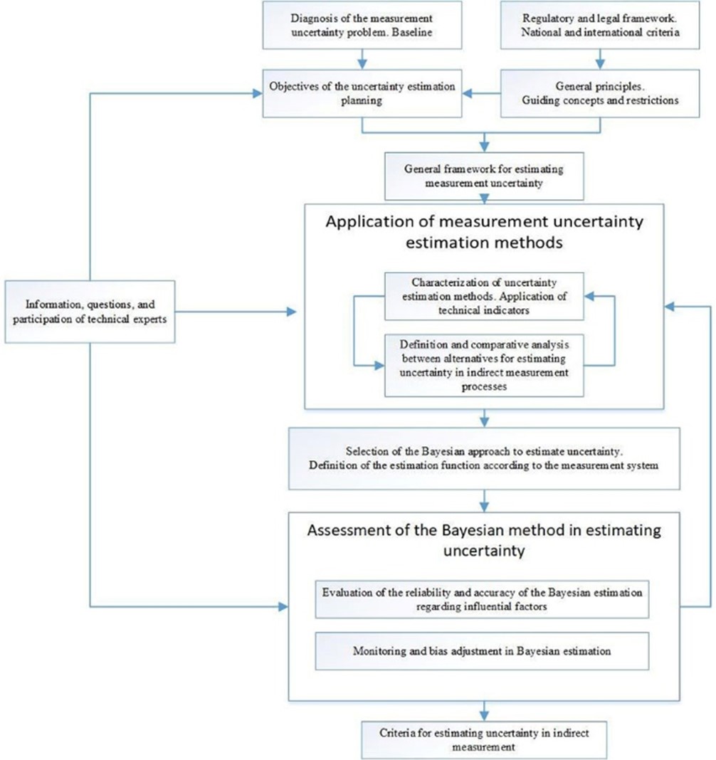
The reliability and accuracy of its results in an indirect measurement must be evaluated to select the Bayesian approach. These aspects are dependent on and linked to the measurement conditions of the instrument used to measure the dependent quantity (multimeter). In this regard, the Bayesian method makes it possible to monitor and adjust the bias associated with the multimeter, thus establishing the criteria for tuning and estimating uncertainty in an indirect measurement system.
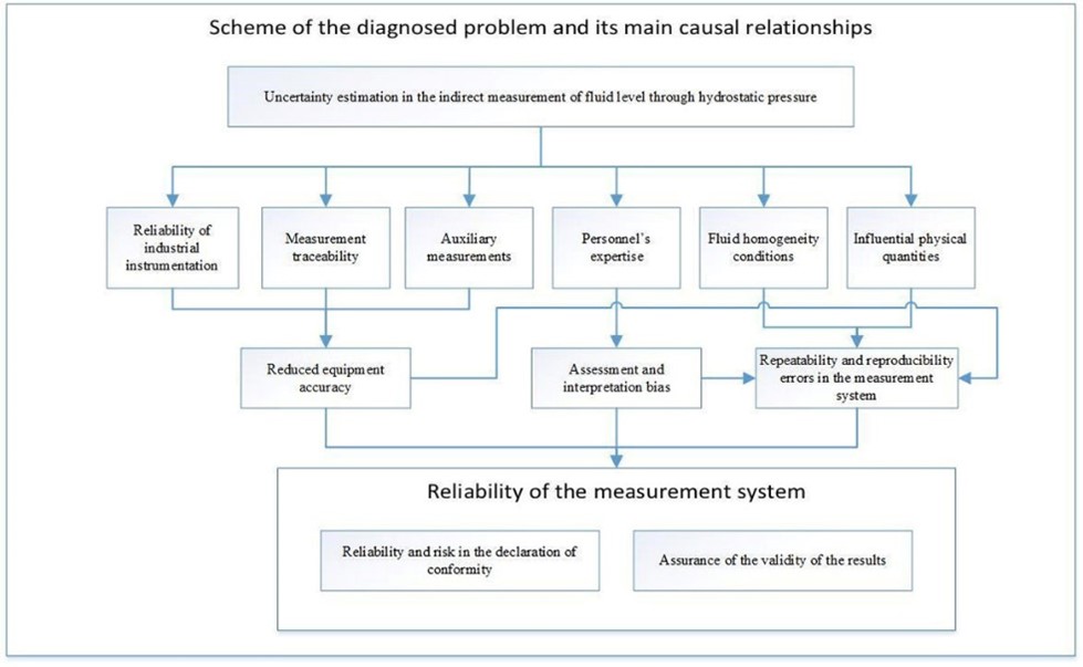
Since the methodological and conceptual scheme shown in Figure 1 constitutes a reference point to estimate uncertainty as per the selected method, the diagnosed problem and its main causal relationships should be outlined as a starting point. Therefore, Figure 2 illustrates the problem’s scheme for the case under study, which serves as input for the implementation of the uncertainty estimation methods, from which the best expression that defines the reliability of the measurement system is determined.
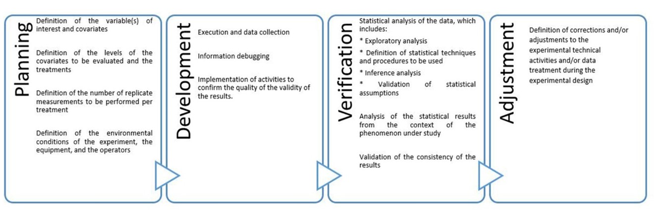
An organized experimental design was developed to conduct each analysis in this study. This design was, in turn, accompanied by a statistical analysis that supports the quality of the validity of the results and confirms the accuracy of applying the uncertainty estimation methods.
The measurement uncertainty associated with the results provided by the multimeter (as an indirect measuring instrument) significantly depends on its precision, the bias observed after its calibration, and other related aspects such as drift, resolution, and intrinsic errors. For this reason, the characteristics having a significant correlation with the instrument, as well as those that do not cause atmospheric pressure changes that may affect the results of the transmitter were identified.
Figure 3 presents the phases that ensure the validity of the results, which contributes to the reliability in the selection, nature, and management of the information linked to each of the estimates obtained with the different methods.
Experiment overview
The measurement system under study aims to indirectly measure the level of a fluid at rest in a non-volumetric container. In other words, the fluid height (h) is the measurand or output quantity; and hydrostatic pressure (Ph), fluid density (ρ), and local gravity (g) are the input quantities, as given by Equation (1)[22].
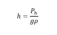 (1)
(1)Local gravity, which is assumed to be constant in this model, was estimated following the ME-017 procedure published by the Centro Español de Metrología (Spanish Metrology Center) (abbreviated CEM in Spanish) [23]. Under the experiment’s conditions,  A Waterpilot FMX21 HART (Highway Addressable Remote Transducer) transmitter consisting of an oil-free ceramic measuring cell was employed. Prior to testing, its zero and span were adjusted as per the physical conditions of the fluid container, which influence the delimitation of the minimum and maximum intervals of both the inlet pressure (0–5 bar), which corresponds to the fluid height inside the tank (0–50 cm), and the output electrical signal (4–20 mA).
Since the test fluid used for the experiment was drinking water, the density-compensated level measurement and integrated temperature measurement (using a PT100 sensor) functions had to be activated. Five reference levels and ten replicate measurements per level were considered, for a total of fifty measurements taken randomly. During the measurements, the following performance characteristics were verified:
- Temperature of the medium: -10–70°C (14–158°F)
- Measurement range: 0–20 bar/200 m H2O (0–300 psi/600 ft H2O), in such a way as to guarantee a deviation of ± 0.2% over the entire measurement scale
- Controlled ambient temperature: 20°C ± 3°C
- Constant inlet and outlet flow rate to ensure that the fluid level remains at rest
- Use of calibrated measuring equipment
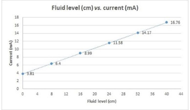
Once the measuring equipment was in working order, its characteristic operating curve was estimated to identify zero, linearity, and angularity errors or any other type of error that may affect the measurement result. Figure 4 illustrates the operating principle of the pressure transmitter in terms of the relationship between the output quantity and the input quantities.
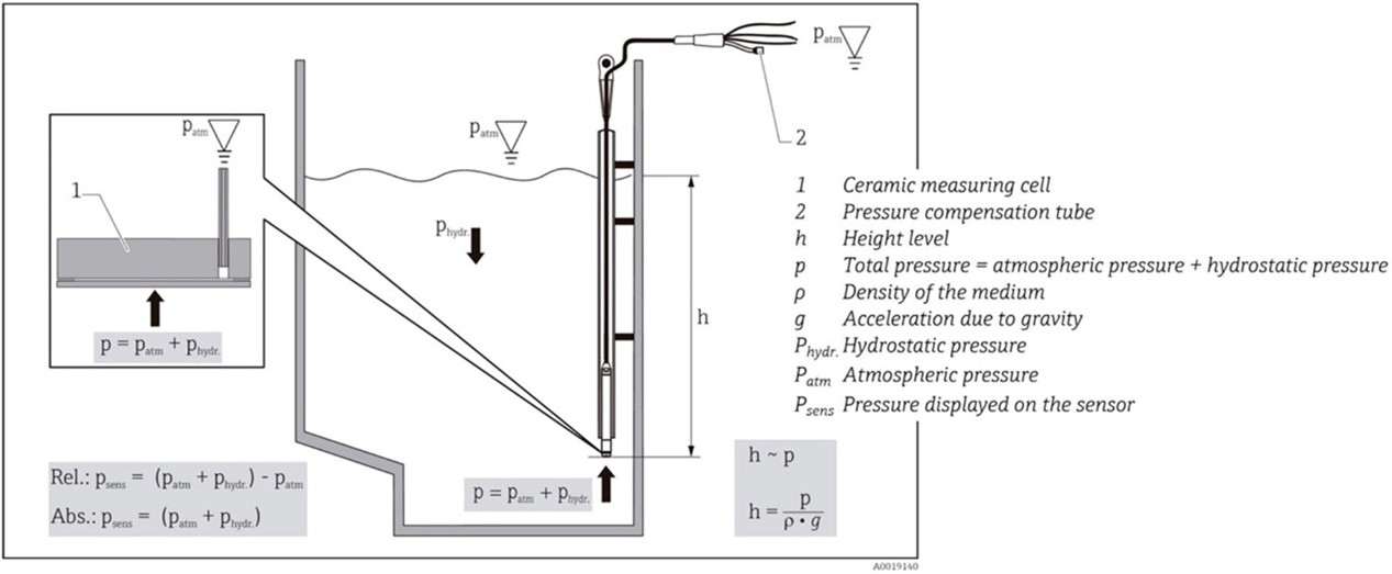
As the transmitter loses linear behavior at pressure values below 0.05 bar, its use is restricted to pressures between 0.1 and 20 bar. The total volume inside the container was divided into five levels representing the heights measured by a Vernier instrument with a resolution of 0.05 mm. The average density of the fluid, which was calculated using the gravimetric method using a class II balance and a class A glass graduated cylinder with a 10-ml hexagonal glass base, was
It was necessary to evaluate repeatability and ensure there were no outliers regarding the factors influencing the measurement results (i.e., operators’ expertise, environmental conditions, procedure, main or auxiliary measuring tools, and measurement time) to consider the resulting measurements valid for this study. The results obtained during the experiment were, thus, confirmed by analyzing two factors: measurement time and personnel in charge of the measurement. Such confirmation aimed to prevent the null hypothesis, which states equality in the results of the experiments carried out at different times and by different personnel, from being rejected. Additionally, the measuring equipment was used per the manufacturer’s operating specifications.
Those characteristics related to the multimeter and associated with uncertainty due to precision, calibration, drift, resolution, and instrument errors (inherent) were established as the inputs or factors leading to variations in the uncertainty of the measurand.
This study’s measurement uncertainty estimation analysis includes comparing the results obtained with the Bayesian approach with those obtained with the GUM and the MC method. The outcome of such a comparison would make it possible to test the null hypothesis (H0) that the Bayesian approach provides more useful information than the other two methods. In addition, it would contribute to the study of the reliability of the measurement process and, above all, to improving uncertainty estimation.
Estimating measurement uncertainty using the Guide to the Expression of Uncertainty
Once the physical model was defined, the factors influencing the uncertainty of the measurand were evaluated. Figure 5 outlines the deterministic model proposed by the GUM. For the case under study, this model represents the statistical analysis of the series of observations that comprise the repeatability of the measurement system, as well as the characterization, quantification, and dispersion of the sources of uncertainty that propagate and are associated with the resulting deviation of the indirect measurement.
The statistical analysis was carried out using, as a reference point, the standardized ME-017 procedure set forth by the CEM [23]. Hence, the uncertainty estimates are given in units of pressure and, according to the existing proportionality between hydrostatic pressure and fluid level, the results are presented in units of length. Likewise, uncertainty due to variation in the pressure gauge reading, or Type A uncertainty (Uα), was estimated, with this being the component that defines the standard variation in the meter reading under process repeatability conditions. The expression used to calculate Type A uncertainty is given by Equation (5).
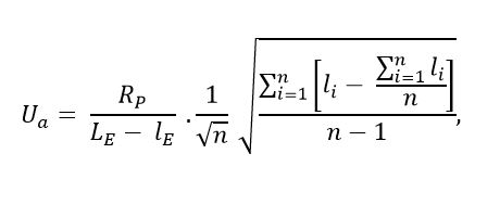 (5)
(5)where Rp is the instrument’s measurement range given in units of pressure; LE, the highest value of the electrical range; lE, the lowest value of the electrical range; li, the indication value of the multimeter for a given nominal pressure; and n, the number of measurements considered. According to the GUM, this is the only source of uncertainty considered to be of Type A.
After estimating Type A uncertainty, the Type B uncertainty sources were established. Here, the indirect measurement was carried out by calculating the electrical current (mA in DC) at the output of the differential pressure transmitter. This value is proportional to the pressure exerted by the fluid on the bottom of the tank, which, in turn, depends on the fluid level inside it. For this reason, the energy meter’s contribution to uncertainty must be estimated using the multimeter’s calibration certificate, and this source must be considered to be of Type B, as follows:
a) Type B uncertainty due to the calibration of the multimeter, : It corresponds to the measurement of the electrical signal, which, assuming a normal distribution, will be given by Equation (6)[23]
 (6)
(6)where k is the coverage factor (Joint Committee for Guides in Metrology, 2008); and UcertE the uncertainty stated in the energy meter’s calibration certificate. If the measurement uncertainty of the multimeter (in mA) is not specified in its calibration certificate, the mathematical function of uncertainty reported by the calibration laboratory is used [23].
b) Type B uncertainty due to the drift of the multimeter, : It is largely associated with the use conditions and maintenance of the measuring equipment. If the historical calibration data of the instrument are assumed to follow a rectangular distribution (which is expected in the variable under study), Equation (7) is applied [23].
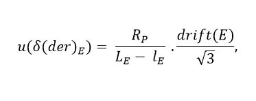 (7)
(7)where drift (E) is the maximum difference in absolute value between the corrections obtained for the meter in two consecutive calibration certificates. When there is only one calibration record, the equipment manufacturer's specifications can be employed [23].
c) Uncertainty due to the instrument’s resolution, : It is due to the scale division of the transducer for each measurement, which will be at least that of the multimeter. If the data are assumed to follow a rectangular distribution, this uncertainty is estimated through Equation (8)[23].
 (8)
(8)where res (E) is the resolution of the measuring instrument.
d) Uncertainty due to the hysteresis of the meter, : It is considered an uncertainty factor because the measurement result can vary depending on whether the value of the variable to be measured is increased or decreased. For a rectangular distribution, this uncertainty is calculated as shown in Equation (9)[23].
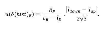 (9)
(9)where Idown corresponds to the mean of the values measured in a downward direction, while Iup denotes the mean of the values measured in an upward direction.
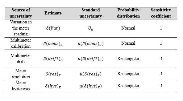
Given the stable environmental conditions in the laboratory and the repeatability of the density result in each stack of experiments oriented to estimate measurement uncertainty using the GUM, uncertainty due to fluid density was not considered here. As an uncertainty budget, Table 1 provides a summary of the factors considered in the measurement uncertainty estimation and their characteristics.
Once the Type A and Type B uncertainties were estimated, the combined uncertainty was calculated, which is defined by Equation (10) for the case under study.
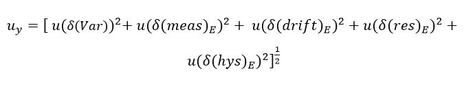 (10)
(10)The sources of uncertainty driven by the factors influencing the measurement, such as hydrostatic pressure (Ph), fluid density (ρ), and local gravity (g), are synergistically considered in Equation (10) because they are embedded in the analysis of the instrument used to measure the dependent quantity (multimeter), which gives increasing importance to the indirect measurement. It should be noted that the covariances of correlated arguments between the factors were estimated, and the result was zero. When any interaction between the factors or sources of uncertainty was observed, the random selection of the correlated parameters or factors at different levels was verified. Then, the expanded uncertainty was calculated using Equation (4). It was necessary to estimate the effective degrees of freedom that guaranteed the validity of the coverage factor (with k =2) and a confidence level of 95.45% using the Welch–Satterthwaite equation (3).
Estimating measurement uncertainty using the Monte Carlo and adaptive Monte Carlo methods
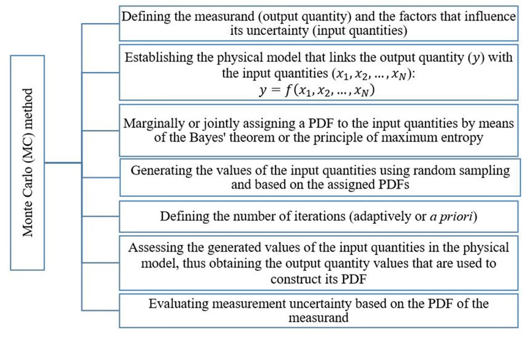
Figure 6 illustrates the sequence to estimate measurement uncertainty using the MC method. This method employs probabilistic schemes and mathematical models to mimic the random behavior of a measurement system, thus making it possible to analyze the risks that uncertainty estimation poses to itself.
Like the GUM, the MC method draws upon a previously defined physical model (which links the output quantity with the input quantities), as expressed in Equation (1), to assign PDFs to the input quantities.
The estimated uncertainty of the measurand was discriminated by five reference levels of fluid height (8 cm, 16 cm, 24 cm, 32 cm, and 40 cm) considering the experimental conditions of this study. Although, in theory, hydrostatic pressure (Ph) and fluid density (ρ) are directly proportional [22], a hypothesis in which they are assumed as independent is proposed in this study because the fluid used for the experiment was drinking water and, during the process, its density did not change significantly. The global average density of the fluid employed for the experiment was  with a sample standard deviation of
  and a coefficient of variation of around 0.17%, which is considerably small. To validate the hypothesis of independence between Ph and ρ, Hoeffding’s test [25] was used through the statistical software R [26]. In (11) are presented the hypotheses to be verified with such test:
 (11)
(11)where F (Ph, ρ) denotes the joint Cumulative Distribution Function (CDF) of Ph and ρ; and G (Ph) and H (ρ), the marginal CDFs of Ph and ρ, respectively. With H 0, the aim is to validate that Ph and ρ are independent. After performing the test globally (considering all observations values and discriminating by reference level), H 0 could not be rejected in all cases, which is why it is concluded that Ph and ρ can be assumed as independent.
Moreover, a hypothesis was formulated to verify that the input quantities marginally followed a normal distribution. To test this hypothesis, the Shapiro–Wilk test [27] was applied globally using all the data for ρ and discriminating observations by reference level for Ph. The null hypothesis that the data followed a normal distribution was not rejected in all cases. For ρ, 50 data were available, while, for Ph, the computation was made using 10 data from each reference level.
Subsequently, the values of the input quantities were generated via random sampling using R [26]. The respective PDFs of the input quantities for each reference level were entered into this software, and the number of iterations (M) was set to 1x10⁶ The generated values of the input quantities were evaluated in the model that links the output quantity with the input quantities, thus obtaining, for each reference level M, values for the output quantity. With this, the mean, standard deviation, coverage interval, and PDF of the measurand were calculated at each reference level.
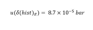
In addition to estimating uncertainty with the MC method, experiments were also conducted using a technique derived from this method and known as adaptive MC. This latter seeks to define the number of iterations necessary for each reference level to guarantee the stabilization of the results. The number of significant figures was set to 2 to define the numerical tolerance. In addition, given the magnitude of the standard deviation of the measurand at each level, numerical tolerance (δ) was set to 0.05 cm. After applying the adaptive MC technique in each reference level of the measurand, results were found to stabilize, in all cases, with a number of iterations below 1x10⁶.
Estimating measurement uncertainty using the Bayesian approach
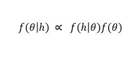
Figure 7 presents the Bayes’ theorem for estimating uncertainty in measurement systems based on intrinsic knowledge. Equation (12) shows how the posterior distribution of the parameters of interest is calculated within this figure, where the estimation of the measurement uncertainty is based.
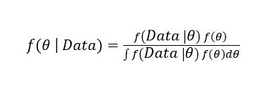 (12)
(12)
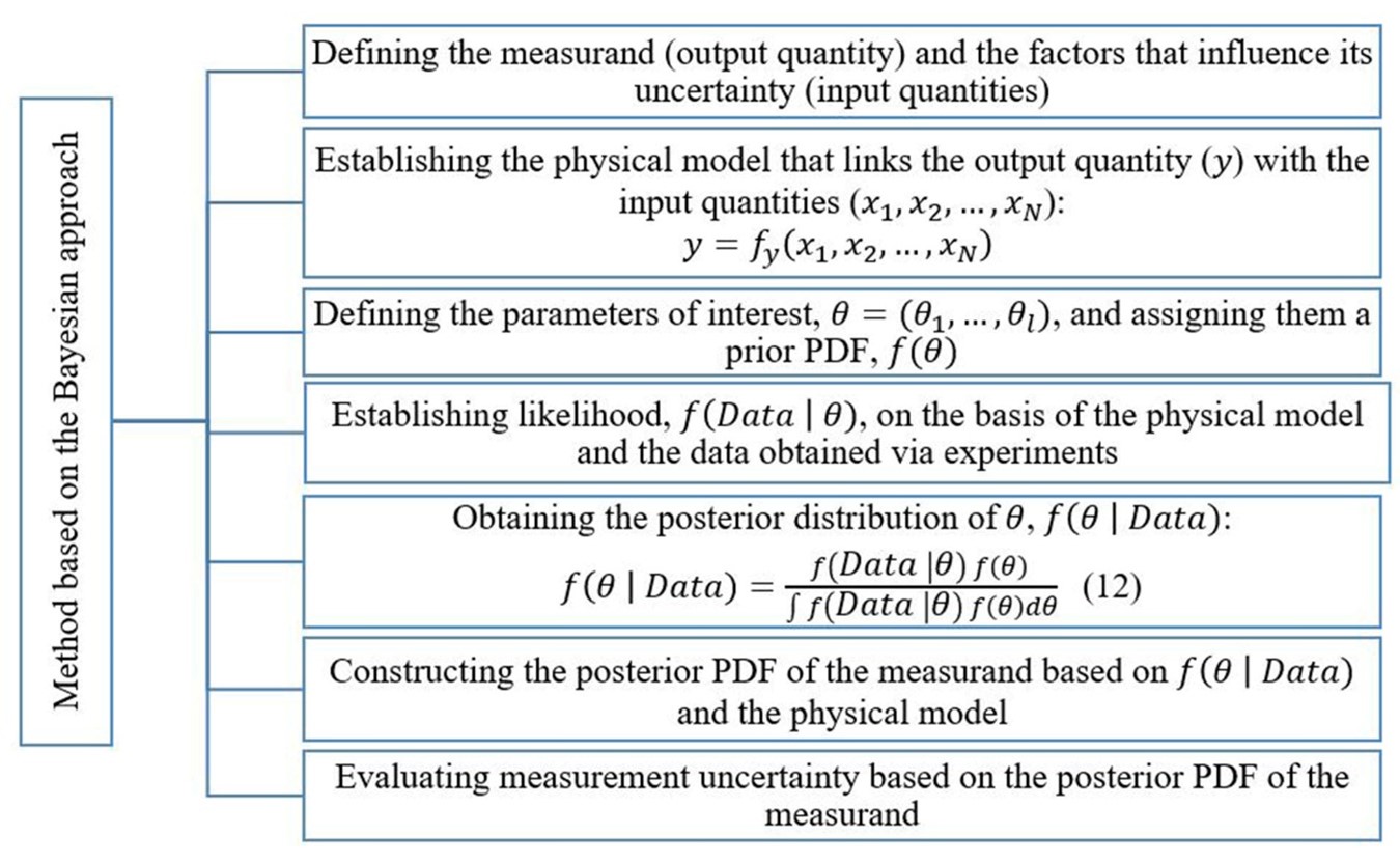
The Bayesian method must also draw upon the physical model that links the output quantity with the input quantities. Experimental data that are representative of the phenomenon and validated should be available. In addition, assigning prior distributions requires familiarity with the conditions and characteristics of the phenomenon under study. In particular, for the case under study, the estimation of measurement uncertainty via the Bayesian approach must be discriminated by the reference level of fluid height. First, we consider the likelihood function presented in (13).
 (13)
(13)where Ph and ρ are independent. By assuming local gravity as constant, we obtain that , and that each observation value of the fluid height,
  has a distribution with probability density function, as is presented in (14)[28].
 (14)
(14)where  is the cumulative standard normal distribution function; and α(hi), b(hi), c and d(hi), the substitution blocks given by the equations presented in (15).
 (15)
(15)
 and be the vectors of the parameters of interest and observations, respectively. Since the observations are independent of each other (because each observation value represents a replica of the experiment), the likelihood function
 would be written as Equation (13).
 (16)
(16)Subsequently, prior distributions must be assigned to the parameters related to the input quantities. Given that the density of water is, in theory, expected to be and that there is no considerable variability in the density of the fluid used (drinking water), we assume that
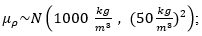 ; therefore,

In addition, we set
For the parameters related to hydrostatic pressure, we consider that Ph = gph; hence, for each level with a reference value (href) in meters, we assume that and
and 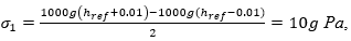 , where g is the value of gravity; Pa, the unit in pascals, with the following conversion formula:
  ; and U, the uniform distribution. We state that
 on the understanding that if a fluid density value is established, the variation in the hydrostatic pressure measurement will not generate a fluid height value that differs by more than 2 cm from the real value. In this case, we assume that
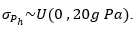
Assuming independence between the parameters,  is equal to the product of the prior marginal PDFs. Thus, the posterior distribution of θ could be written as is presented in (17).
 (17)
(17)For the experimental testing of the case under study, values for  were generated via the Markov Chain Monte Carlo (MCMC) method using the t-walk algorithm [29]. A total of 1.1 x 10⁶ values were produced, with an initial burn-in of 1x10⁵ values. Finally, by replacing the generated values of θ in the model that links the output quantity with the input quantities, the posterior PDF of the measurand was obtained.
Results
Results obtained with the Guide to the Expression of Uncertainty in Measurement
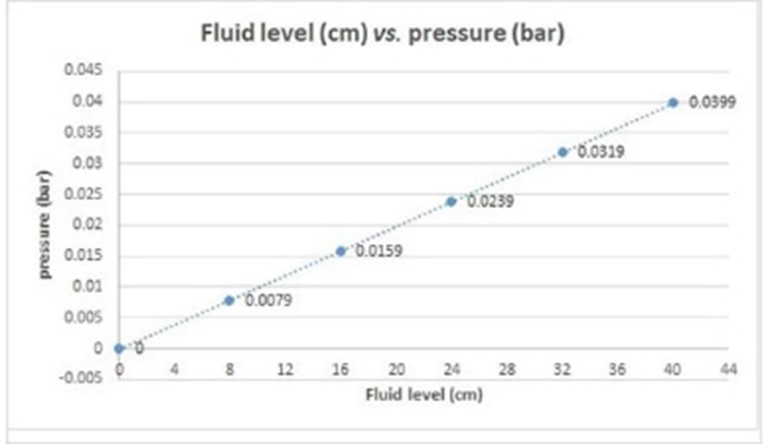
Figures 8 and 9 show the directly proportional relationship between pressure (represented by the transmitter’s output signal in mA) and fluid height.
Using Equation (5), the Type A uncertainty, which indicates the standard variation in the pressure transmitter reading under process repeatability conditions, is calculated, thus obtaining the result presented in (18).
 (18)
(18)As the first source of Type B uncertainty, the energy meter’s calibration, whose coverage factor is removed to obtain a value as real as possible. Applying Equation (6), we get the result presented in (19).
 (19)
(19)Another source of Type B uncertainty is the drift of the multimeter, , which is estimated using Equation (7). Considering the information provided by the manufacturer regarding the accuracy of the equipment for electrical current measurements (± 0.8 mA DC, which is equivalent to 0.128 mA), we obtain the result presented in (20).
 (20)
(20)To estimate the uncertainty due to the multimeter’s resolution, Equation (8) is employed, where res(E) corresponds to the resolution of the electrical indication for the meter, which, in this case, is 0.01 mA DC. We get the result presented in (21).
 (21)
(21)Using Equation (9), the uncertainty due to the hysteresis of the meter is calculated, thus obtaining the result presented in (22).
 (22)
(22)Then, the combined uncertainty and the expanded uncertainty are estimated using Equations (10) and (4), respectively. Thus, we get the results presented in (23).
 (23)
(23)Table 2 presents the results of estimating measurement uncertainty using the GUM, which were discriminated by the reference level of fluid height and expressed in height units. Here, SD corresponds to the standard deviation. In addition, the proportionality between fluid height and pressure was established (see Figure 9) by dividing the uncertainty estimate in the pressure measurement by the product of the average density of the fluid for a given reference level and local gravity. All this was done considering the necessary unit conversions to convert the results to centimeters (cm).
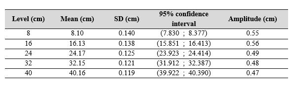
As observed in Table 2, the mean values of the measurand were close to the nominal values (consistently above 0.1 cm) in all cases. In addition, the standard deviation estimates fluctuated around 0.2 and 0.1 cm at the different levels, and the confidence intervals always contained the nominal value of the reference level.
Results obtained with the Monte Carlo and adaptive Monte Carlo methods
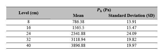
Table 3 reports the parameters estimated for Ph per reference level (a mean of  and a standard deviation of
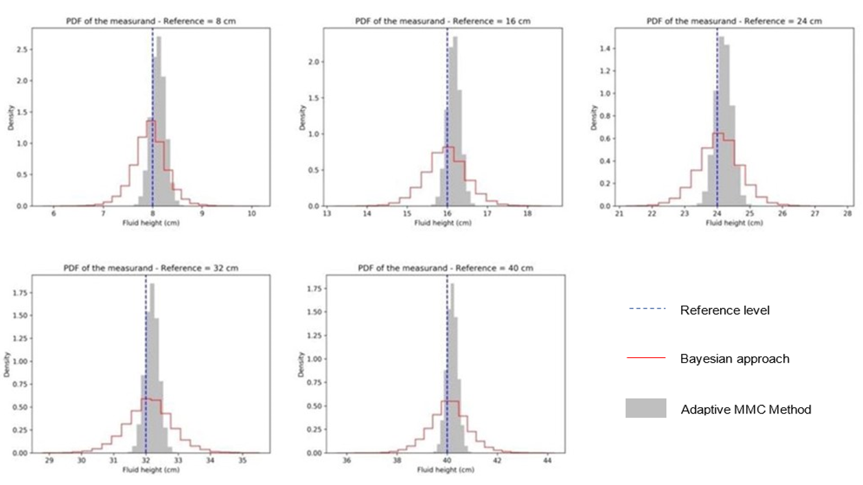
  were assigned for ρ). Table 4 shows the mean, standard deviation, and coverage interval estimates, while Figure 10 illustrates the PDF of the measurand for each reference level.
Results obtained with the Bayesian approach
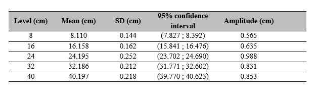
Table 5 presents the results obtained based on the posterior PDF of the measurand for each reference level.
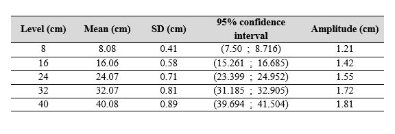
As shown in Table 5, the mean values of the measurand at each reference level of fluid height were close to the nominal value of the corresponding level, with a difference between the estimate and the reference value below 0.8 cm. In all cases, the standard deviation was below 1 cm, and the amplitude of the coverage intervals was always less than 2 cm. In addition, the coverage interval contained the reference value in each reference level. Finally, Figure 10 compares the PDFs of the measurand for each reference level, obtained with the Bayesian approach and the adaptive MC method.
Conclusions
This paper aimed to validate a methodology (illustrated in Figures 1, 2, and 3 above) that can be used as a guide to applying techniques showing a good performance in estimating measurement uncertainty (e.g., the GUM, the MC method, and the Bayesian approach). This methodology provides conceptual elements that make it possible to understand and analyze the functional contribution of several techniques when applied to a non-trivial case study that has been little examined in the literature.
In particular, the results of estimating uncertainty in an indirect measurement system via the Bayesian approach were compared with the estimates obtained with the GUM and the MC method. The case under study sought to calculate the fluid level by measuring its hydrostatic pressure at rest on the bottom of a container. According to the findings, there are differences between the uncertainty estimates obtained with the methods implemented and discussed here, which serve as criteria when deciding which to use. The GUM, for instance, provides estimates for calculating the mean and standard deviation of a measurand, in addition to its confidence interval. For their part, the MC and Bayesian techniques offer complementary information (such as the PDF of a measurand) that may be more useful in a given case. Through this PDF, the analysis can be expanded by estimating the mean, the standard deviation, the median, the mode, the quantiles, the symmetry, and the coverage interval of the measurand. The difference between the PDF obtained with the MC method and that obtained with the Bayesian approach is that this latter technique offers a posterior PDF that can be updated if new information is available.
Furthermore, based on the adaptive MC method, the application of the GUM in the case under study was found to be adequate, which is explained by the fact that the model that links the output quantity with the input quantities follows a simple behavior. In other words, the PDF of the measurand was found to be symmetric and bell-shaped in each reference level, which was also observed when both the MC and Bayesian approaches were applied. This confirms the assumption that the GUM is based when it is assumed that the PDF of the measurand is normal or approximately normal.
A contribution derived from the structure of the experiments presented in this study (such as the application of the GUM, the MC method, and the Bayesian approach in a non-trivial phenomenon with industrial applicability and not frequently addressed in the literature) was to demonstrate the ability of the Bayesian approach to provide results closer to an accurate measurement compared to those offered by the GUM and the MC method. This numerical precision of the Bayesian approach was attributed to the fact that the PDFs of the measurand obtained for each reference level assigned the highest probability to the interval that contained the nominal or actual value. Additionally, one of the theoretical advantages of the Bayesian approach is the possibility to update or refine the inference model as new data are available. Moreover, with this approach, the intervals of possible values for the measurand are wider than those offered by the MC method and the GUM.
References
[1] Joint Committee for Guides in Metrology, Evaluation of measurement data – guide to the expression of uncertainty in measurement, BIPM, 2008. [Online]. Available: https://www.bipm.org/documents/20126/2071204/JCGM_100_2008_E.pdf/cb0ef43f-baa5-11cf-3f85-4dcd86f77bd6
[2] T. Dietza, K. Klamrothb, K. Kraus, et al., “Introducing multiobjective complex systems,” European Journal of Operational Research, vol. 280, no. 2, pp. 581-596, 2020. https://doi.org/10.1016/j.ejor.2019.07.027
[3] C. Cai, J. Wang and Z. Li, “Assessment and modelling of uncertainty in precipitation forecasts from TIGGE using fuzzy probability and Bayesian theory,” Journal of Hydrology, vol. 577, 2019. https://doi.org/10.1016/j.jhydrol.2019.123995
[4] T. B. Schön, , A. Svensson, L. Murray and F. Lindsten, “Probabilistic learning of nonlinear dynamical systems using sequential Monte Carlo,” Mechanical Systems and Signal Processing, vol. 104, pp. 866-883, 2018. https://doi.org/10.48550/arXiv.1703.02419
[5] T. Hou, D. Nuyens, S. Roles and H. Janssen, “Quasi-Monte Carlo based uncertainty analysis: Sampling efficiency and error estimation in engineering applications,” Reliability Engineering and System Safety, vol. 191, 2019. https://doi.org/10.1016/j.ress.2019.106549
[6] Joint Committee for Guides in Metrology, JCGM 101:2008 – Evaluation of measurement data - Supplement 1 to the “Guide to the expression of uncertainty in measurement” – Propagation of distributions using a Monte Carlo method, BIPM, 2008.
[7] J. M. M. R. Roberto Arias R., “Determinación de la incertidumbre de medición del volumen de patrones volumétricos, determinado a partir del método de pesado de doble sustitución,” Santiago de Querétaro, 2002.
[8] M. A. Azpurua, C. Tremola and E. Paez, “Comparison of the gum and Monte Carlo methods for the uncertainty estimation in electromagnetic compatibility testing,” Progress In Electromagnetics Research B, vol. 34, pp. 125 - 144, 2011. https://doi.org/10.2528/PIERB11081804
[9] S. F. dos Santos and H. S. Brandi “Application of the GUM approach to estimate uncertainty in measurements of sustainability systems,” Clean. Techn. Environ. Policy, 2015. https://doi.org/10.1007/s10098-015-1029-3
[10] K. Weise and W. Woger, “A Bayesian theory of measurement uncertainty,” Meas. Sci. Technol, vol. 4, no. 1, 1992. https://doi.org/10.1088/0957-0233/4/1/001
[11] I. Lira, “The GUM revision: The Bayesian view toward the expression of measurement uncertainty,” European Journal of Physics, vol. 37, no. 2, p. 025803, 2016. [Online]. Available: https://iopscience.iop.org/article/10.1088/0143-0807/37/2/025803
[12] D. G. I Lira, “Bayesian assessment of uncertainty in metrology: a tutorial,” Metrologia, nº 47, pp. R1 - R14, 2010. [Online]. Available: https://iopscience.iop.org/article/10.1088/0026-1394/47/3/R01
[13] J.-H. Y. Heung-Fai Lam, “An innovative Bayesian system identification method using autoregressive model,” Mechanical Systems and Signal Processing, vol. 133, 2019. https://doi.org/10.1016/j.ymssp.2019.106289
[14] J. Berger, “The case for objective Bayesian analysis,” Bayesian Analysis, vol. 1, nº 3, pp. 385- 402, 2006. https://doi.org/10.1214/06-BA115
[15] L. S. Katafygiotis, “Sequential Bayesian estimation of state and input in dynamical systems using output-only measurements,” Mechanical Systems and Signal Processing, vol. 131, pp. 659-688, 2019. https://doi.org/10.1016/j.ymssp.2019.06.007
[16] I. Lira and W. Wöger “Bayesian evaluation of the standard uncertainty and coverage probability in a simple measurement model,” Measurement Science and Technology, vol. 12, no. 8, pp. 1172 –1179, 2001. [Online]. Available: https://iopscience.iop.org/article/10.1088/0957-0233/12/8/326/meta
[17] F. Attivissimo, N. Giaquinto and M. Savino, “A Bayesian paradox and its impact on the GUM approach to uncertainty,” Measurement, vol. 45, no. 9, pp. 2194-2202, 2012. https://doi.org/10.1016/j.measurement.2012.01.022
[18] C. Elster and Blaza Toman, “Bayesian uncertainty analysis under prior ignorance of the measurand versus analysis using the Supplement 1 to the Guide: a comparison,” Metrología, vol. 46, no. 3, pp. 261 – 266, 2009.
[19] M. Vilbaste, G. Slavin, O. Saks, V. Pihl and I. Leito, “Can coverage factor 2 be interpreted as an equivalent to 95% coverage level in uncertainty estimation? Two case studies,” Measurement, vol. 43, no. 3, pp. 392–399, 2010. https://doi.org/10.1016/j.measurement.2009.12.007
[20] A. Possolo, “Five examples of assessment and expression of measurement uncertainty,” Applied Stochastic Models Bussines and Industry, vol. 22, no. 1, pp. 1-18, 2012. https://doi.org/10.1002/asmb.1947
[21] A. Gelman, J. Carlin, H. Stern and D. Rubin, Bayesian data analysis, Boca Raton, FL, USA: Chapman & Hall/CRC, 2014.
[22] F. White, Fluid Mechanics, 6th Ed., McGraw-Hill, 2008.
[23] Centro Español de Metrología, Procedimiento ME - 017 para la calibración de transductores de presión con salida eléctrica, Madrid, España, 2003.
[24] Endress+Hauser. (2015). Technical Information Waterpilot FMX21. https://portal.endress.com/wa001/dla/5000557/8038/000/05/TI00431PEN_1413.pdf
[25] W. Hoeffding, “A non-parametric test of independence,” The annals of mathematical statistics, vol. 19, no. 4, pp. 546-557, 1948. https://doi.org/10.1214/aoms/1177730150
[26] R Core Team, “R: A language and environment for statistical computing,” R Foundation for Statistical Computing, Vienna, Austria, 2017.
[27] S. S. Shapiro and M. B. Wilk, “An analysis of variance test for normality (complete samples),” Biometrika, vol. 52, no. 3/4, pp. 591-611, 1965. https://doi.org/10.2307/2333709
[28] T. Pham-Gia, N. Turkkan and E. Marchand, “Density of the ratio of two normal random variables and applications,” Communications in Statistics-Theory and Methods, vol. 9, no. 35, pp. 1569-1591, 2006. https://doi.org/10.1080/03610920600683689
[29] J. A. Christen and F. Colin, “A general purpose sampling algorithm for continuous distributions (the t-walk),” Bayesian Analysis, vol. 2, no. 5, pp. 263-281, 2010. https://doi.org/10.1214/10-BA603
Notes
*
Report of case
Author notes
a Corresponding author. E-mail: juan.molina@cimat.mx
Additional information
How to cite this article: J. D. Molina-Muñoz, L.F. Giraldo-Jaramillo, E. Delgado-Trejos, “Bayesian evaluation for uncertainty of indirect measurements in comparison with GUM and Monte Carlo” Ing. Univ. vol. 26, 2022. https://doi.org/10.11144/Javeriana.iued26.beui
