


APA
ISO 690-2
Harvard
Haga clic en un formato de citación
Criterion to Determine the Sample Size in Stochastic Simulation Processes*
Criterio para determinar el tamaño de muestra en procesos de simulación estocástica
Juan Daniel Molina-Muñoz, José Andrés Christen
Criterion to Determine the Sample Size in Stochastic Simulation Processes*
Ingeniería y Universidad, vol. 26, 2022
Pontificia Universidad Javeriana
Juan Daniel Molina-Muñoz a juan.molina@cimat.mx
Centro de Investigación en Matemáticas, México
José Andrés Christen
Centro de Investigación en Matemáticas, México
Received: 04 december 2020
Accepted: 10 august 2021
Published: 29 july 2022
Abstract: Objective: To propose a criterion to determine the sample size in stochastic simulations of MC (Monte Carlo) and MCMC (Markov chain Monte Carlo), guaranteeing certain precision estimating parameters. It is intended that the accuracy is guaranteed in a dimensionless way. Materials and methods: This paper proposes a criterion is proposed that seeks to meet the stated objective. In addition, a methodology for its application. Results and discussion: The application of the methodology is presented in 3 different contexts: MC simulation in which the sample of interest presents moderate variability, MC simulation in which the sample of interest presents excessive variability, and MCMC simulation. In all cases, adequate estimates of the number of MC and MCMC runs are obtained from relatively small samples. Furthermore, the application of the methodology represents only a marginal additional computational cost. Conclusions: The criterion presented in this paper allows for determining the sample size in stochastic simulations, guaranteeing dimensionless precision in estimating parameters.
Keywords:Stochastic simulation, sample size, Monte Carlo, MCMC, coefficient of variation.
Resumen: Objetivo: Proponer un criterio para determinar el tamaño de muestra en simulaciones estocásticas de MC (Monte Carlo) y MCMC (Markov chain Monte Carlo), garantizando una determinada precisión en la estimación de parámetros. Se busca que la precisión se garantice de forma adimensional. Materiales y métodos: El presente artículo propone un criterio buscando cumplir con el objetivo planteado. Además, de una metodología para la aplicación del mismo. Resultados y discusión: Se presenta la aplicación de la metodología en 3 contextos diferentes: Simulación de MC en que la muestra de interés presenta variabilidad moderada, simulación de MC en que la muestra de interés presenta variabilidad excesiva y simulación de MCMC. En todos los casos se obtienen adecuadas estimaciones del número de corridas MC y MCMC a partir de muestras relativamente pequeñas. Además, la aplicación de la metodología representa únicamente un costo computacional adicional marginal. Conclusiones: El criterio presentado en este artículo permite determinar el tamaño de muestra en simulaciones estocásticas, garantizando precisión adimensional en la estimación de parámetros.
Palabras clave: Simulación estocástica, tamaño de muestra, Monte Carlo, MCMC, coeficiente de variación.
Introduction
The MC (Monte Carlo) simulation method is based on the principle of random sampling; it mainly allows: Generating values of a probability distribution of interest, performing numerical integration (commonly used for parameter estimation), or developing optimization processes [1], [2], [3], [4]. The MCMC (Markov chain Monte Carlo) simulation method is part of the MC family of methods. It is especially useful when we want to simulate values of a complex multidimensional probability distribution, and possibly its normalization constant is not explicitly known. This situation is common in the context of Bayesian statistics, without being the exclusive area of application of the method [5], [6], [1]. In general, the tools offered by the MC and MCMC methods help modeling physical, economic, biological, medical, and social phenomena, which makes these methods widely used in multiple areas of knowledge [7], [8], [9], [10], [11].
In the execution of MC simulations, or stochastic simulation (with or without MCMC), a fundamental decision determining the sample size (or a number of simulations to be performed). The importance of this decision stems from the fact that the sample size influences the estimation error of quantities of interest (QoI) and the precision of the estimates made. It could be thought of as a solution to reduce error by having a sample size as large as possible. However, each new simulation has a computational cost that will depend on the system’s complexity of the to be simulated. For this reason, there is an interest in constructing a criterion that would allow finding the optimal sample size necessary to guarantee a given precision in the estimation of parameters.
In the development of stochastic simulation processes, a common practice is to set the sample size with values considered more or less “standard” (100 or 1000 or 10,000 or 1 ∙ 10^6 or others). These become “magical numbers” that, although accepted in many academic settings, do not guarantee precision in the estimation of parameters or in the control of the simulation error. This practice is fairly common, as can be seen for example in these recent publications: [11], [12], [10], [13], [9].
Although the theory is straightforward, applying the Central Limit Theorem (CLT) to build confidence intervals and classical sample sizes, surprisingly, there are not many published alternatives with the details to determine the sample size in an MC simulation quantitatively. For example, in [4] (p. 139), which is a widely known book in the area of stochastic simulation, the following procedure is proposed to set the simulation sample size:
Choose an acceptable value for the standard deviation of the estimator of a parameter of interest.
Generate a sample of the variable of interest of size at least 100.
Continue generating additional values, stop when k values have been generated and  , where represents the sample standard deviation of the generated values.
The method proposed by [4] can be considered arbitrary in setting the initial sample size to at least 100. Furthermore, the choice of the d value is ambiguous.
Some popular stochastic simulation books do not present an explicit criterion to determine the sample size in MC simulations, but limit themselves to proposing the use of the CLT and confidence intervals to evaluate the convergence of the estimators, with little emphasis on the details [1], [14].
In the case of MCMC simulations, most of the literature present criteria to guarantee the convergence of the chain made up of the simulated values. However, no specific criteria are presented to ensure precision in the estimates calculated under convergence conditions [5], [1]. One of the few alternatives is the criterion proposed in [15] to determine burn-in in MCMC simulations and the sample size necessary to guarantee precision in estimating a quantile of a function of the model parameters.
The papers on this topic primarily represent applications in specific knowledge areas. In many of these papers, the methods they use to calculate the sample size are based on the confidence interval formula for the mean that follows from the CLT, and the expression of the width of the interval, the sample size is obtained. The variation of each method resides on which set of the following elements they assume fixed or known: The confidence level, the width of the interval, the admissible estimation error, and the coefficient of variation [16], [17], [18], [19], [20], [21], [22]. However, in most cases, it is not intuitive to determine a suitable value for the width of the interval or the allowable estimation error. Regarding the coefficient of variation, the situations in which it is known in advance are almost zero. Furthermore, the sample size calculation depends on this value, a circular estimation argument is incurred in the case of estimating the mean.
This paper presents a criterion to determine the sample size of a stochastic simulation (with or without MCMC), which guarantees a certain precision (established by the user) in estimating the parameters. The important factor is that such precision is guaranteed in a dimensionless way based on the number of “significant figures” that the MC estimator has. That is, let  expressing this number in scientific notation, we have the result presented in equation (1).
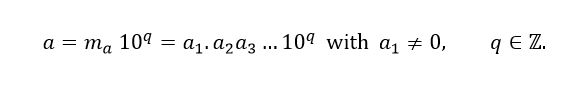 (1)
(1)Indeed, mα is the mantissa of α, by convention  to guarantee a unique representation of α, α1.α2α3 is the decimal expansion of mα and the q exponent. The user establishes how many significant numbers p needs/wants to be correct with a probability close to 1 (>0.9999) in an MC estimator of α. In that case, q and α1 to αp would be correct, with a probability of 0.9999. An algorithm is proposed for the implementation of the criterion, simple and of negligible computational cost, through a preliminary estimation of the coefficient of variation (Cv, the standard deviation divided by the expected value of a functional of interest). It should be mentioned that the mathematical contribution of the methodology proposed in this paper is rather marginal; as said before, it is well known how the sample size in an MC estimator should be proposed using the CLT. The value of this paper is in going through the details, using as a unique criterion the number of significant figures in an estimator, the overall practical utility of the resulting method, and its computational simplicity.
This paper is organized as follows: First, the criterion proposed to determine the sample size is exposed, a methodology is proposed to implement the criterion, and considerations are presented to determine of the sample size in the case of an MCMC simulation. Later, multiple illustrative examples of the proposed methodology are developed. Finally, the conclusions are presented.
Materials and methods
Notation and definition of the criterion
Let  be a random variable with probability density function (or mass probability)
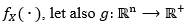 , be a positive functional. We considered the values presented in equation (2).
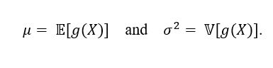 (2)
(2)It is desired to estimate μ from a MC simulation of X. Let X1, X2, ..., XT be a sample of independent and identically distributed variables of  obtained from MC simulation. Considering the estimator for μ, we use the simple mean presented in equation (3).
 (3)
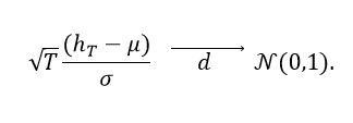
(3)By the central limit theorem [23] we have the result presented in equation (4).
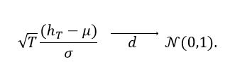 (4)
(4)Expressing μ in scientific notation as in (1), we have that μ is equal to what is shown in equation (5).
 (5)
(5)Now, taking the exponent of μ, we consider ht and σ expressed as is shown in equation (6).
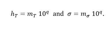 (6)
(6)Note that mT and mσ are not necessarily the mantissas of the scientific notation convention described in (1). Then (2) can be rewritten as is presented in equation (7).
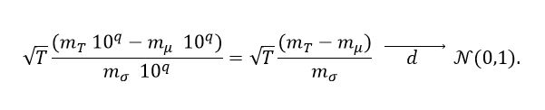 (7)
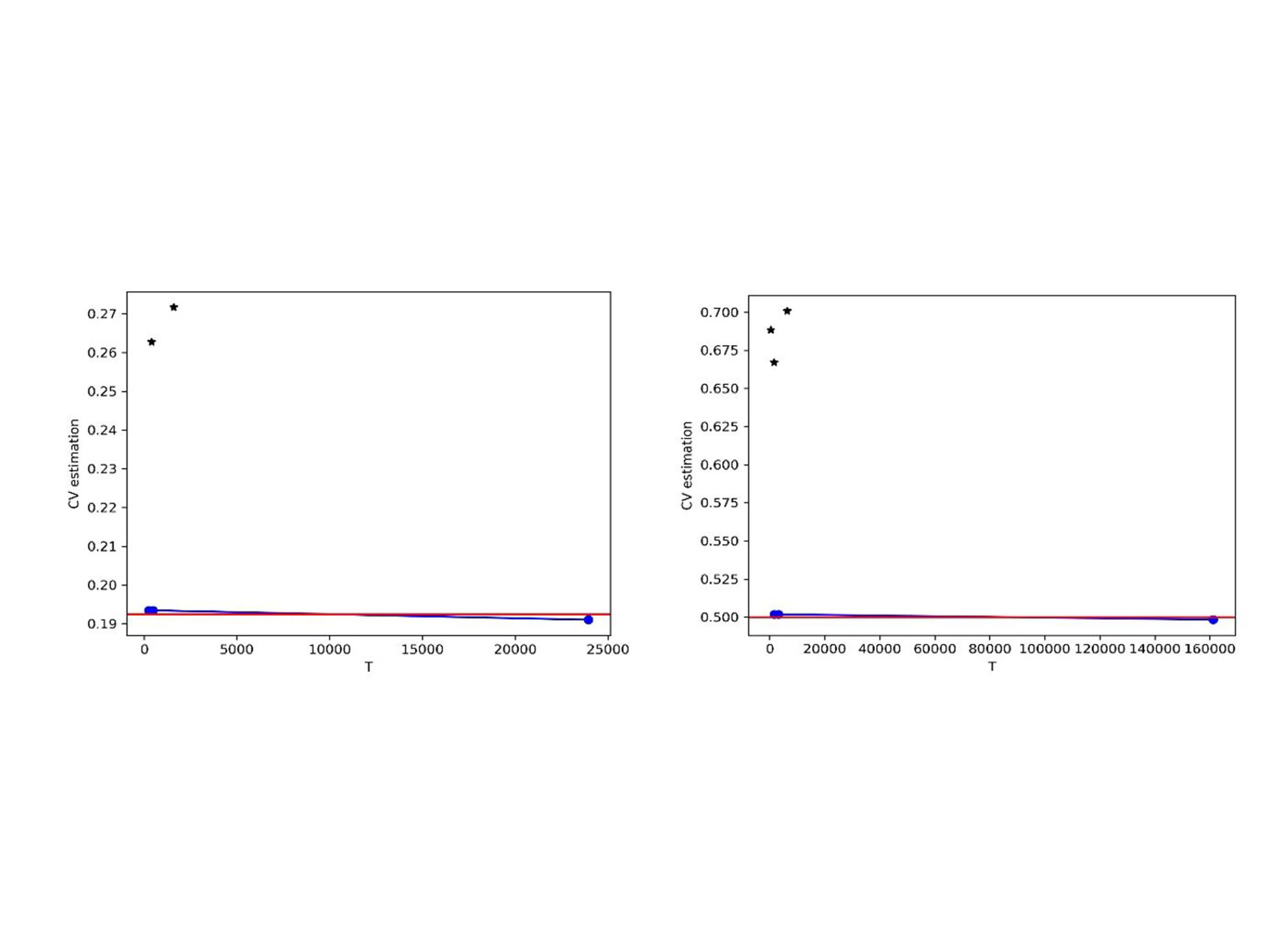
(7)Now, let  be an established value, the interest is given in guaranteeing with high probability (close to 1) a precision of p significant figures in the estimation of the mantissa of mμ, that is, that mμ = mT if both quantities are rounded to p significant figures. Which happens if the inequality presented in equation (8) is satisfied.
 (8)
(8)To guarantee the result (4) are considered the calculations presented in equation (9).
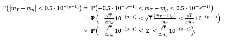 (9)
(9)the latter considering the result (3), with Z a random variable such that  In this way, we have that
  a quantile of the Z distribution such that
  Taking z = 4, we have
Therefore, the minimum sample size that guarantees a precision of p significant figures in the estimate of mμ is the expression presented in equation (10).
 (10)
(10)Now, considering that  that is, 𝓂σ = Cv 𝓂μ, we have that
  But 𝓂μ <10, being a mantissa, then
  with which the result presented in equation (11) is obtained.
 (11)
(11)A standard case is when in this case the expression (5) is equivalent to the expression presented in equation (12).
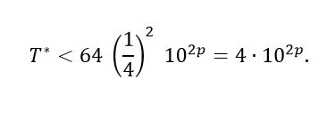 (12)
(12)Now, assuming that we have T independent simulations of a functional of interest, to determine the precision that this number of runs guarantees in the estimation of mμ, we can start from the expression (5), make T = 64 Cv2 102p and from this equality obtain p, the resulting expression is shown in equation (13).
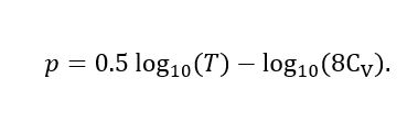 (13)
(13)Thus, the p that is calculated by means of expression (6) represents an upper bound for the precision that can be guaranteed in the estimation of mμ, of the functional with T simulations. Thus, we may fix a precision p and calculate the required T* or with a given current number of samples T calculate the actual number of significant figures p in an estimator.
In general, the coefficient of variation  cannot be estimated directly, since in this way a circular argument is incurred with respect to the main objective of guaranteeing precision in the estimation of mμ. It is then proposed to make a preliminary (rough) estimate of the Cv in which all the sample information is not used. This preliminary estimation is proposed to be carried out by means of the Bland method [24], which is presented in Appendix A.
Correction for MCMC
Let X1, X2, ... be a reversible Markov chain. Let as is shown in equation (14).
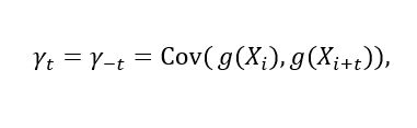 (14)
(14)the autocovariance in the lag t of the reversible time series g(X1), g(X2), ..., [25] explain that for a stationary, irreducible and reversible Markov chain we have the result presented in equation (15).
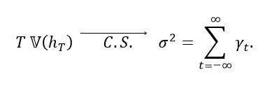 (15)
(15)Furthermore, if  we have the result equation (16).
 (16)
(16)That is, expression (7) represents the central limit theorem for the case of dependent samples constructed from a stationary, irreducible, and reversible Markov chain. In [26], a method to estimate σ2, is proposed, which is presented in Appendix B.
Thus, given the result presented in (7), the results proposed in the previous section are equally valid for samples constructed via MCMC. It should be noted that the definition and interpretation of σ2, changes between the case of the simulation of an independent sample via MC to the case of the simulation of a dependent sample via MCMC.
In the MCMC case, to avoid incurring a circular argument when estimating the Cv, there are 2 alternatives: First, estimate the integrated autocorrelation time (IAT) of the sample and, from this, extract the dependent sample into a pseudo-independent sample and on the latter, apply the procedure outlined in the next section. The second option is, given that the circular argument falls only on μ and that this parameter is estimated in the same way for independent and dependent samples, it is proposed to estimate μ by means of Bland's method [24] and σ, using Geyer's method [26]. For this last alternative applying the procedure proposed in the next section to estimate T* is valid, except for the change in the estimation of σ,
Heuristic method to calculate T*
An iterative methodology is proposed to calculate the T* that guarantees a precision of p significant figures:
Let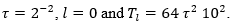 Generate via Monte Carlo simulation a sample of independent variables of the functional of interest of size Tl, and from this calculate
  which represents the estimate of Cv by means of the Bland method.
While  Generate a sample of independent variables of the functional of interest of size Tl
, and from this calculate
Generate a sample of independent variables of the functional of interest of size Tl
, and from this calculate 
If τ > 4 print the message "The procedure stops because the sample of interest has excessive dispersion" and stop the algorithm. If not, continue with the next step.
Make  (with
(with  the last estimator calculated by means of Bland's method). Generate a sample of independent variables of the functional of interest of size Tl, and from this calculate
  (traditional estimator). Make
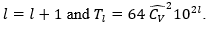
While generate a sample of independent variables of the functional of interest of size Tl, and from this calculate
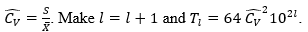
Return T* = Tp.
With steps 1 and 2 of the algorithm the Cv preliminary estimation of the is structured. The function of τ is to define a suitable upper bound for Cv. Initially,  is assumed, which represents the standard or regular case, if this assumption is not feasible
  , is assumed and so on, multiplying the bound by 2. The last scenario considered in the preliminary estimation is
  With steps 4 and 5 of the algorithm, the estimation of the Cv is refined, using all the available sample information.
For greater efficiency, it is recommended that in each step of the algorithm that is required to generate a sample of independent variables of  , not to discard the values that have previously been generated. Taking into account that in this way, at no time, is the assumption of independence between the elements of the sample violated.
If we have an independent sample of the functional of interest of size T and on this we want to calculate the precision p that is guaranteed in the estimation of mμ, the previous algorithm is still valid. It is only necessary that, in each of the steps, when talking about generating a sample of size Tl, it is taken from the available sample. In this case, the algorithm stops at the moment that Tl> T and the precision that is guaranteed is p = l - 1.
Python implementation
The algorithm explained in the previous section was implemented in Python. Two functions were defined for both MC simulations and MCMC simulations:
One that calculates the sample size T* necessary to guarantee p precision in estimating the mantissa of a functional of interest; the arguments that this function receives are the desired precision, the sample generation mechanism and the functional one; this function returns the value of T*, a sample of size of T* the functional of interest, estimates in the initial and refinement stage of the coefficient of variation and the sample size, and gives an estimate of μ (calculated on the sample of size T*) in scientific notation by rounding its mantissa to p significant figures.
The other allows to calculate the precision that is guaranteed for a certain sample; the argument of this function is the sample to evaluate; this function returns the value of the number p of significant figures that can be guaranteed with the sample, and an estimate of μ in scientific notation by rounding its mantissa with p significant figures.
The Python codes with the algorithm implementation along with the examples presented in this paper may be found on the GitHub platform, at the link: https://github.com/jdmolinam/Sample_Size_Criterion
Results
Three examples were developed to present the application of the algorithm proposed in different conditions. Example 1 presents the case in which the coefficient of variation of the functional of interest is less than  This can be considered a standard case of reasonable dispersion. In example 2, the functional has a greater dispersion since it has a coefficient of variation greater than
  Finally, example 3 presents the algorithm application in the context of an MCMC simulation where the true value of the coefficient of variation of the functional of interest is not known in advance.
Monte Carlo simulation with Cv< ¼
Let  Under these conditions we have that the Xi are independent of each other and
  Therefore, the probability density function of X is as is presented in equation (17).
 (17)
(17)Considering the functional  we have for μ the expression (18),
 (18)
(18)and for σ2 the expression (19).
 (19)
(19)Therefore, 
Now, we proceed to calculate an upper bound for the sample size T* that guarantees precision in the estimation of mμ of p =3 significant figures. Developing the iterative process proposed above, it was found  Figure 1 shows the different sample sizes and estimates of the Cv considered in the estimation process of T*. A random sample was generated by MC simulation of size T*, and from this
  , was obtained, that is,
  Thus, remembering that
 In addition, if we round both
  and
and  to 3 significant figures, we have
  Therefore, the precision of p = 3 significant figures in the estimate of
  is confirmed.
Monte Carlo simulation with Cv> ¼
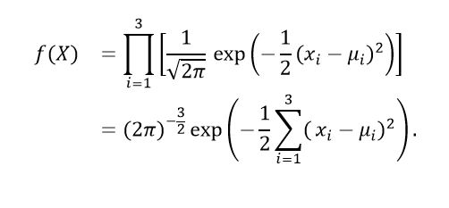
Let X = (X1, X2, X3, X4) with X1, X2, X3, X4 independent and identically distributed so that Therefore, the probability density function of X is as is presented in equation (20).
 (20)
(20)Considering the functional  , we have μ for the expression (21),
 (21)
(21)and σ2 for the expression (22).
 (22)
(22)Therefore,
Now, we proceed to calculate an upper bound for the sample size T* that guarantees precision in the estimation of mμ of p = 3 significant figures. Developing the iterative process proposed above, it was found T* = 15,965,508, figure 1 shows the different sample sizes and estimates of the Cv considered in the estimation process of T*. A random sample was generated by MC simulation of size T*, and from this,  was obtained, that is,
  Thus, remembering that
  we have that
  In addition, if we round both
  and
and  to 3 significant figures, we have
 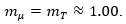 Therefore, the precision of p = 3 significant figures in the estimate of
  is confirmed.
*On the left the results of example 1 and on the right those of example 2. The asterisks represent the estimates of CV in the initial stage and points the estimates in the refinement stage
MCMC simulation: Bayesian estimation in the Lotka–Volterra model
This example was developed around the Lotka–Volterra system of equations, which describes the dynamics of two populations of animals: one predator and one prey. The system was considered under the conditions presented in equation (23).
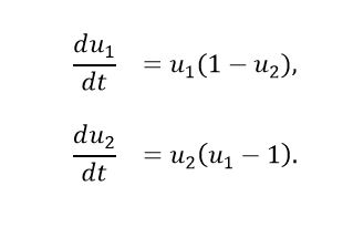 (23)
(23)Where 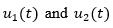 represent the population (thousands of specimens) at time t of the prey and predator species respectively.
  are unknown. The parameters that characterize the model are
  and of these, the parameter of interest is
  Thus, the functional to consider is
An inverse Bayesian problem is posed [27], in which the available data have the structure presented in equation (24).
 (24)
(24)with  Thus,
Thus,  For the simulation of the data was set
 with observations taken on the times {0.75, 1.5, 2.25, 3.0, 3.75}. The prior distribution presented in equation (25) was considered.
 (25)
(25)with e = 0.2. In this way, we have as is shown in equation (26).
 (26)
(26)Let Y = (y1, ..., yn) be the vector of observations, the likelihood function is characterized by the expression (27).
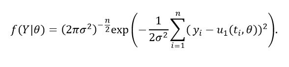 (27)
(27)Thus, the posterior distribution is determined by Bayes’ theorem, that is: 
Under the conditions of this example, the parameter on which we want to guarantee precision in our estimation is
 (28)
(28)The MCMC algorithm t-walk [28] was used to generate values of the posterior distribution. Initially, 10,000 iterations were run, from which it is stated that with a burn-in of 500 iterations, the chain made up of the simulated values reaches the stationary state.
Now, we proceed to calculate an upper bound for the sample size T* that guarantees precision in estimating  of p = 2 significant figures. The proposed procedure was developed with the exception of making the preliminary estimation of the coefficient of variation by estimating the mean with the Bland method and the standard deviation of the dependent sample with the Geyer method. T* = 942,270 was obtained. Figure 2 shows the posterior distributions obtained from an MCMC sample size T*.
Additionally, Table 1 shows the precision guaranteed for each of the examples in the case in which there is a sample of size T (independent in examples 1 and 2, obtained via MCMC in 3) of the functional of interest. The precision calculation was made using the proposed heuristic algorithm, assuming Cv unknown.
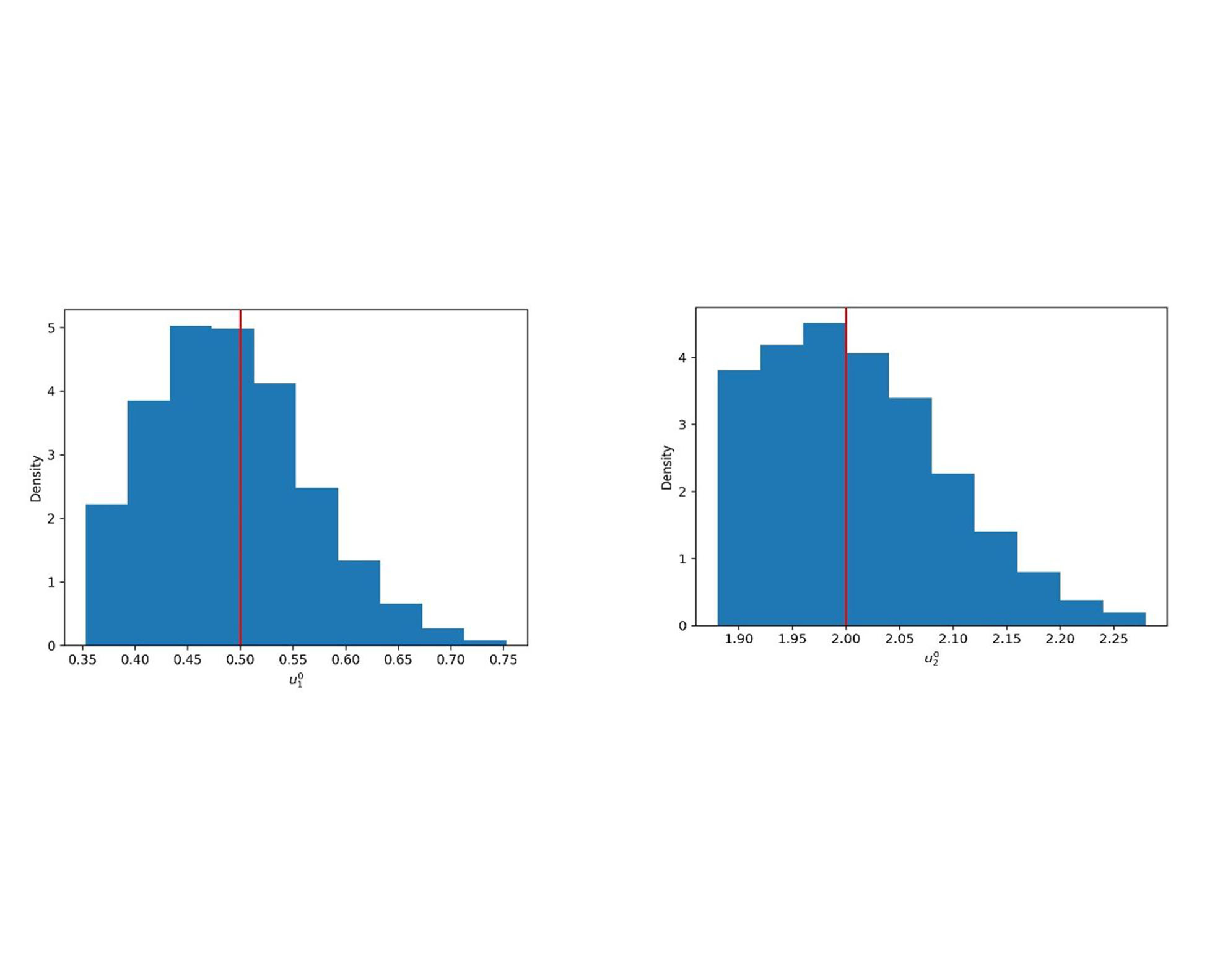
*On the left the posterior distribution of  on the right that of
  The red lines at
  represent the values of the parameters used to generate the synthetic data.
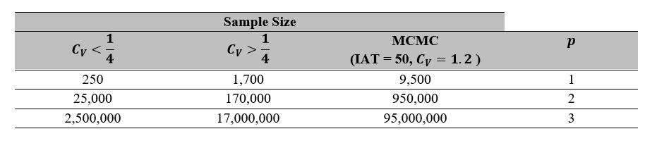
* In the case  the different accuracies are guaranteed with smaller sample sizes, for the case
  larger samples are required and in the MCMC case much more. Thus, arbitrarily choosing the sample size with “magical numbers” in general is an error, which is exacerbated if we have a
  or usually for MCMC simulations. Note the well-known, and commonly neglected, 100 times increase in sample size with one significant figure increase in precision, resulting from the ½ convergence rate in the CLT.
Conclusions
In many cases, the problem of determining the sample size in stochastic simulations is approached superficially using “magical numbers”, or using techniques that do not offer guarantees, such as the control of the simulation error or precision in the estimation of parameters. This represents a severe problem, especially if we have a  or if an MCMC simulation is performed where the IAT is greater than 1, which is the case in most common non-trivial cases.
The criterion presented in this paper allows determining the sample size in stochastic simulations, guaranteeing dimensionless precision in estimating parameters. The importance of this result does not lie in its mathematical contribution but its practical value.
The heuristic methodology presented in this paper for applying the criterion in each application example proved to be efficient as it does not require large initial samples to make a good preliminary estimate of Cv and T*. Furthermore, this methodology does not add a great computational cost to the overall simulation process. The authors consider that implementing this methodology in commonly used statistical software such as R and Python would become a very useful tool.
References
[1] C. Robert and G. Casella, Monte Carlo statistical methods, Springer Science & Business Media, 2004, https://doi.org/10.1007/978-1-4757-4145-2
[2] G. Fishman, Monte Carlo: concepts, algorithms, and applications, Springer Science & Business Media, 2013.
[3] J. S. Liu, Monte Carlo strategies in scientific computing, Springer Science & Business Media, 2008, https://doi.org/10.1007/978-0-387-76371-2
[4] S. Ross, Simulation, 5th ed., Elsevier Science, 2012.
[5] D. Gamerman and H. F. Lopes, Markov chain Monte Carlo: stochastic simulation for Bayesian inference, Chapman and Hall/CRC, 2006.
[6] B. A. Berg and A. Billoire, Markov chain Monte Carlo simulations, Wiley Encyclopedia of Computer Science and Engineering. Wiley Online Library, 2007.
[7] C. Forastero, L. Zamora, D. Guirado a A. Lallena, “A Monte Carlo tool to simulate breast cancer screening programmes,” Physics in Medicine & Biology, vol. 55, no. 17, p. 5213, 2010, https://doi.org/10.1088/0031-9155/55/17/021
[8] H. MacGillivray, R. Dodd, B. McNally, J. Lightfoot, H. Corwin and S. Heathcote, “Monte-Carlo simulations of galaxy systems,” Astrophysics and Space Science, vol. 81, no. 1-2, pp. 231-250, 1982, https://doi.org/10.1007/BF00683346
[9] T. Flouri, X. Jiao, B. Rannala and Z. Yang, “A Bayesian implementation of the multispecies coalescent model with introgression for phylogenomic analysis,” Molecular Biology and Evolution, vol. 37, nº 4, pp. 1211-1223, 2020, https://doi.org/10.1093/molbev/msz296
[10] C. L. Ritt, J. R. Werber, A. Deshmukh and M. Elimelech, “Monte Carlo simulations of framework defects in layered two-dimensional nanomaterial desalination membranes: implications for permeability and selectivity,” Environmental Science & Technology, vol. 53, nº 11, pp. 6214-6224, 2019, https://doi.org/10.1021/acs.est.8b06880
[11] I. Ciufolini and A. Paolozzi, “Mathematical prediction of the time evolution of the COVID-19 pandemic in Italy by a Gauss error function and Monte Carlo simulations,” The European Physical Journal Plus, vol. 135, nº 4, p. 355, 2020, https://doi.org/10.1140/epjp/s13360-020-00383-y
[12] R. Al, C. R. Behera, K. V. Gernaey and G. Sin, “Stochastic simulation-based superstructure optimization framework for process synthesis and design under uncertainty,” Computers & Chemical Engineering, Vol. 143, pp. 107-118, 2020, https://doi.org/10.1016/j.compchemeng.2020.107118
[13] E. Spitoni, K. Verma, V. S. Aguirre and F. Calura, “Galactic archaeology with asteroseismic ages-II. Confirmation of a delayed gas infall using Bayesian analysis based on MCMC methods,” Astronomy & Astrophysics, vol. 635, p. A58, 2020, https://doi.org/10.1051/0004-6361/201937275
[14] O. Jones, R. Maillardet and A. Robinson, Introduction to scientific programming and simulation using R, Chapman and Hall/CRC, 2014.
[15] A. E. Raftery and S. Lewis, How many iterations in the gibbs sampler? In J. M. Bernardo, M. J. Bayarri, J. O. Berger, A. P. Dawid, A. F. M. Smith, eds., Bayesian Statistics, vol. 4, Oxford University Press, 1992.
[16] I. Lerche and B. S. Mudford, “How many Monte Carlo simulations does one need to do?,” Energy exploration & exploitation, vol. 23, no. 6, pp. 405-427, 2005, https://www.jstor.org/stable/43754693
[17] F. E. Ritter, M. J. Schoelles, K. S. Quigley and L. C. Klein, “Determining the number of simulation runs: Treating simulations as theories by not sampling their behavior,” in L. Rothrock and S. Narayanan (eds.), Human in the loop simulations, Springer, 2011, pp. 97-116.
[18] M. Liu, “Optimal Number of Trials for Monte Carlo Simulation,” VRC-Valuation Research Report, 2017.
[19] L. T. Truong, M. Sarvi, G. Currie and T. M. Garoni, “How many simulation runs are required to achieve statistically confident results: a case study of simulation-based surrogate safety measures,” 2015 IEEE 18th International Conference on Intelligent Transportation Systems, 2015, pp. 274-278, https://doi.org/10.1109/ITSC.2015.54
[20] G. Hahn, “Sample Sizes for Monte-Carlo Simultation,” IEEE Transactions on Systems Man and Cybernetics, no. 5, p. 678, 1972. https://ieeexplore.ieee.org/stamp/stamp.jsp?arnumber=4309200
[21] W. Oberle, Monte Carlo Simulations: Number of Iterations and Accuracy, Army Research Lab Aberdeen Proving Ground Md Weapons and Materials Research, 2015, https://apps.dtic.mil/sti/pdfs/ADA621501.pdf
[22] M. D. Byrne, “How many times should a stochastic model be run? An approach based on confidence intervals,” Proceedings of the 12th International conference on cognitive modeling, Ottawa, 2013.
[23] R. J. Serfling, Approximation theorems of mathematical statistics, John Wiley & Sons, 2009.
[24] M. Bland, “Estimating mean and standard deviation from the sample size, three quartiles, minimum, and maximum,” International Journal of Statistics in Medical Research, vol. 4, no. 1, pp. 57-64, 2014, https://doi.org/10.6000/1929-6029.2015.04.01.6
[25] C. Kipnis and S. S. Varadhan, “Central limit theorem for additive functionals of reversible Markov processes and applications to simple exclusions,” Communications in Mathematical Physics, vol. 104, no. 1, pp. 1-19, 1986, https://doi.org/10.1007/BF01210789
[26] C. J. Geyer, “Practical markov chain Monte Carlo,” Statistical Science, vol. 7, no. 4, pp. 473-483, 1992, https://doi.org/10.1214/ss/1177011137
[27] M. A. Capistrán, J. A. Christen and S. Donnet, “Bayesian analysis of ODEs: solver optimal accuracy and Bayes factors,” SIAM/ASA Journal on Uncertainty Quantification, vol. 4, no. 1, pp. 829--849, 2016, https://doi.org/10.1137/140976777
[28] J. A. Christen and C. Fox, “A general purpose sampling algorithm for continuous distributions (the t-walk),” Bayesian Analysis, vol. 5, no. 2, pp. 263-281, 2010, https://doi.org/10.1214/10-BA603
Appendix A. Method for the preliminary estimation of the Cv
Given the interest in making a preliminary estimation of the Cv, the Bland method [24] is considered, which allows for estimating the mean and variance of a sample of independent and identically distributed variables without using the total sample information. The method is explained below.
Let X be a random variable in  , with probability density function (or mass probability)
 be a sample of independent and identically distributed variables of
  and let X(1), X(2), ... X(n) the order statistics of the sample. The following quantities are considered: a=X(1) the first sample quartile, 𝒎 the sample median, q3 the third sample quartile, and b = X(n) Considering that the sample mean and variance are determined by the expressions presented in equation (29).
 (29)
(29)and for simplicity it is assumed 𝒏 = 4Q +1, with Q ∈ ℤ+, that is, Q = (𝒏-1)/4, for the estimation of the sample mean, the inequalities presented in equation (30) are taken into account.
 (30)
(30)Adding all the previous inequalities and dividing by 𝒏 we obtain αp≤͞X≤ βp, where αp is defined as shown in equation (31),
 (31)
(31)and βp as is shown in equation (32).
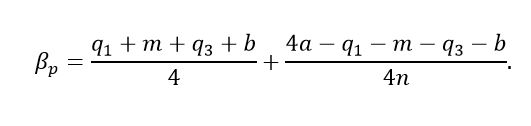 (32)
(32)Then, we have the result presented in equation (33).
 (33)
(33)To estimate the sample variance, the inequalities presented in equation (34) are taken into account.
 (34)
(34)Adding all the previous inequalities and with simple algebra we see that 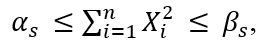 where is defined as shown in equation (35),
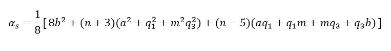 (35)
(35)and βs as is shown in equation (36).
 (36)
(36)It is proposed, 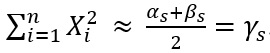 And taking into account the expression (37).
 (37)
(37)Then, we have the result (38).
 (38)
(38)Thus, based on Bland's method, the expression presented in equation (39) is proposed as preliminarily estimation of the Cv
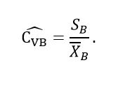 (39)
(39)Normally, a minimal sample size will be needed to obtain an initial rough estimate of Cvusing the above estimator. In the context of the algorithm proposed in this paper, this works well to constrain the estimation problem with an initial bound for Cv using a small trial sample and establish the required sample size.
Appendix B. Method to estimate the variance of a MCMC sample
This appendix presents Geyer's method [26], to estimate the variance of an MCMC sample at stationary state. Considering a reversible Markov chain X1, X2, ..., Let as is shown in equation (40).
 (40)
(40)the autocovariance in the lag t of the stationary time series g(X1), g(X2), ... . This quantity can be estimated from the empirical autocovariance presented in equation (41).
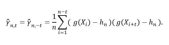 (41)
(41)In [26] it is shown that for a stationary, irreducible and reversible Markov chain, 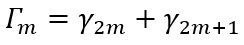 is a strictly positive, strictly decreasing and strictly convex function of 𝒎 Also,
  Based on these results, in [26] the estimator for σ2 presented in equation (42) is proposed.
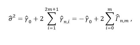 (42)
(42)where 𝒎 is chosen as the largest integer such that the expression (43) is satisfied
 (43)
(43)Notes
*
Research paper - Article of scientific and technological investigation.
Author notes
a Corresponding author. E-mail: juan.molina@cimat.mx. Centro de Investigación en Matemáticas, CIMAT, Guanajuato, México
Additional information
How to cite this article: J.D. Molina Muñoz, J. Christen, “Criterion to determine the sample size in stochastic simulation processes” Ing. Univ. vol. 26, 2022. https://doi.org/10.11144/javeriana.iued26.cdss
